Chapter 17: Creating bar charts using the Histogram utility

Previous chapter                     LLUs Home                     Next chapter

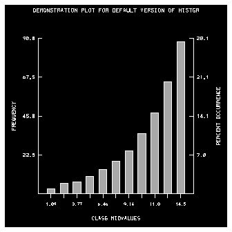
Histograms (bar charts) are used to show the distribution of values in a like-sample dataset. The individual values are sorted by size into a number of value ranges called "class intervals." The number of samples out of the total that fall into a class interval are represented as a histogram bar height. The height of each histogram bar is proportional to the number of samples in that class interval.

Bar chart created using Histogram

Table of Histogram user entry points

There are five user-callable entries within the Histogram utility. HISTGR is called to generate a histogram. HSTOPC, HSTOPI, HSTOPL, and HSTOPR are called before HISTGR to set parameters (options) that affect the output histogram. All parameters have an original default setting.

Action routine

HISTGR

Generates histograms of several types. Raw sample data can be sorted into a default range of classes or an assigned range of classes. Class interval data, which was sorted at an earlier step, can be input and displayed. Two histograms can be displayed simultaneously.

Parameter routines

HSTOPC

Sets parameters of type character, such as titles and labels.

HSTOPI

Sets parameters of type integer, including the color indices to be assigned to the various components of the graphic and the size and orientation of the class (bar) labels.

HSTOPL

Sets parameters of type logical, which is basically an on/off switch for these options.

HSTOPR

Sets parameters of type real, including the location on the plot device where the histogram is to be placed, the spacing of the histogram classes (bars), and if two histograms are present, the overlap of the two.

Table of Histogram parameters

An arbitrary number of options can be set through successive calls to any of the parameter-setting routines. A call to the HISTGR entry will then generate the desired histogram. The four parameter-setting routines are used to set parameters of type character, integer, logical, and real.

For a complete description of the Histogram parameters, see the histogram_params man page.

------------------------------------------------------------------------------------------------
Parameter  Fortran type  Set by  Brief description                  Default value                 
------------------------------------------------------------------------------------------------
FOR        Character     HSTOPC  FORmat for class labels            '(G10.3)'                      
TIT        Character     HSTOPC  A main TITle                       No title                      
LAB        Character     HSTOPC  Class interval axis LABel          'CLASS INTERVALS'                
                                                                    ('MID=OFF')                       
                                                                    'CLASS MIDVALUES'                
                                                                    ('MID=ON')                        
FQN        Character     HSTOPC  FreQueNcy axis label               'FREQUENCY'                      
CHR        Character     HSTOPC  Class interval label string        Internal numeric labels       
COL        Integer       HSTOPI  8 COLorable graphic components     All are white on black        
CLA        Integer       HSTOPI  Size of CLAss labels               Medium size characters        
                                 Orientation of class labels        Horizontal labels             
HOR        Logical       HSTOPL  Direction of histogram bars        Vertical                      
PER        Logical       HSTOPL  A PERcentage axis opposite the     The axis is drawn             
                                 frequency axis                                                   
MID        Logical       HSTOPL  Location of class interval labels  Placed at interval midpoints  
SHA        Logical       HSTOPL  SHAding of histogram bars          Bars are shaded               
DRL        Logical       HSTOPL  Grid lines through bars            No lines are drawn            
MED        Logical       HSTOPL  A line drawn at data MEDian        No line is drawn              
PRM        Logical       HSTOPL  A PeRiMeter around the histogram   No perimeter is drawn         
FRA        Logical       HSTOPL  Advance the FRAme                  The frame is advanced         
LIS        Logical       HSTOPL  LISt parameter values on output    No printed list               
DEF        Logical       HSTOPL  Reset all parameters to DEFaults                                 
WIN        Real          HSTOPR  Region of frame to put histogram   The entire frame              
SPA        Real          HSTOPR  SPAcing between histogram bars     Spacing = 2.0                 
                                 Dual histogram overlap             Overlap = -1.0                
------------------------------------------------------------------------------------------------

Generating a histogram

The HISTGR routine generates histograms for a single data array or compares the histogram distributions of two data arrays. Data values are partitioned into classes. You can make histogram bars represent either the number of occurrences within each class, or a Y-value associated with that class.

A histogram with default options

Code segment 1 from thstgr.f

1       CALL HSTOPL('DEF=ON')
2       CALL HISTGR(DAT1, NDIM, NPTS, IFLAG, CLASS, NCLASS, WORK, NWRK)

Synopsis

 CALL HISTGR (DAT1, NDIM, NPTS,
+ IFLAG, CLASS, NCLASS, WORK, NWRK)

Arguments

DAT1(NDIM,2)

Real, Input---An NDIM by 2 array. See argument IFLAG for a description of input data options.

NDIM

Integer, Input---The first dimension of DAT1.

NPTS

Integer, Input---Number of points to be sorted or number of previously sorted class intervals. The NPTS argument depends on the value of IFLAG:

When IFLAG=0 or 1, NPTS is the number of points in array DAT1 to be sorted into class intervals (bins).

When IFLAG=2 or 3, NPTS is the number of previously sorted class intervals (bins) in array CLASS.

IFLAG

Integer, Input---Used to select one of four histogram options:

0 A single array of length NPTS is loaded into the DAT1 array. HISTGR computes NCLASS equally sized class intervals that vary from the minimum value in DAT1 to the maximum value in steps of
(MAX-MIN)/NCLASS.

The DAT1(NPTS) values are sorted into these bins. The result is a histogram with NCLASS bars (bin counts). The bar height can be labeled by number of points in the bin or by the percentage this is of the total number of points.

1 Similar to IFLAG = 0, except the user can specify the class intervals. For example, the following code sorts DAT1 values into five equally sized bins in the value range from 0. to 10.:

NCLASS = 5
CLASS(1) = 0.
CLASS(2) = 2.
CLASS(3) = 4.
CLASS(4) = 6.
CLASS(5) = 8.
CLASS(6) = 10.

Note: Class intervals need not be equally spaced.

2 To display previously computed histograms, load into the DAT1 array either the number of values in each class interval (bin) or the percentage-of-total value.

NPTS is the number of class intervals (histogram bars). The midpoint value of each class interval is loaded into array CLASS.

For example, the previous example would involve putting a five point histogram in DAT1 and assigning class interval midpoints as follows:

NPTS = 5
CLASS(1) = 1.
CLASS(2) = 3.
CLASS(3) = 5.
CLASS(4) = 7.
CLASS(5) = 9.

3 Similar to IFLAG=2, except two histograms can be displayed for comparison purposes. The first histogram is loaded into DAT1(NPTS,1). The second histogram is loaded into DAT1(NPTS,2). The first histogram can partially shade or obscure the second histogram by the appropriate selection of the SPAC and OVERLP options.

CLASS

Real, Input---Class interval values, dimensioned (NCLASS+1). The CLASS argument depends on the following IFLAG values:

When IFLAG=0, CLASS is not used.

When IFLAG=1, NCLASS+1 class interval endpoints are loaded into array CLASS in a monotonically increasing order. The intervals

need not be of equal width.

When IFLAG=2 or 3, NCLASS midpoint intervals are loaded into array CLASS. They must be in monotonically increasing order, but need not be of equal widths. The histogram bars will, however, be displayed with equal widths.

NCLASS

Integer, Input---Number of class intervals (histogram bars) specified.

WRK

Real, Input---Scratch array dimensioned by NWRK.

NWRK

Integer, Input---The dimension size of array WRK determined from:

NDIM + 3 * (NCLASS + 1)

Discussion

Line 1 of code segment 1 from thstgr.f shows a quick way to reset all internal parameters to their default values. This can be quite useful when you are generating a sequence of histograms that include many parameter-setting calls. It allows you to return every parameter to its default value in a single call. Line 2 generates the histogram.

Comparing two histograms

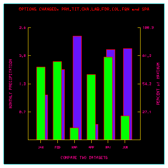
The Histogram utility can be used to compare dual histograms. In the following example, two histograms, each with six class intervals, are compared.

Comparison of two histograms using overlapping bars

Code segment 2 from thstgr.f

1       IFLAG  = 3
2       NCLASS = 6
3       NPTS2  = 2
4       CALL HSTOPL('DEF=ON')
5       CALL HSTOPI('COL=ON',3,0,COLORS,8)
6       CALL HSTOPC('TIT=ON',
       + 'OPTIONS CHANGED: PRM,TIT,CHA,LAB,FOR,COL,FQN and SPA',7,3)
7       CALL HSTOPL('PRM=ON')
8       CALL HSTOPC('FQN=ON','MONTHLY PRECIPITATION',7,3)
9       CALL HSTOPC('FOR=ON','(F3.0)',9,3)
10      MON='JANFEBMARAPRMAYJUNJULAUGSEPOCTNOVDEC'
11      CALL HSTOPC('CHR=ON',MON,12,3)
12      CALL HSTOPC('LAB=ON','COMPARE TWO DATASETS',7,3)
13      SPAC(1) = 2.0
14      SPAC(2) = -1.5
15      CALL HSTOPR('SPA=ON',SPAC,2)
16      CALL HISTGR(DAT1, NDIM, NPTS2, IFLAG, CLASS, NCLASS, WORK, NWRK)

Discussion

Lines 1, 2, and 3 of code segment 2 from thstgr.f set arguments for the HISTGR call. Line 1 sets IFLAG=3 to tell HISTGR that two histograms will be displayed. Line 2 sets NCLASS=6 to specify that six midpoint intervals will be loaded into array CLASS. Line 3 sets NPTS2=2 to specify that that the second histogram is being input in array DAT1(NDIM,NPTS2).

Line 4 resets all internal parameters to their default values.

Line 5 assigns colors to the eight components of the graphic. (Specific colors are not shown since this document is not produced in color.)

Line 6 creates a main title that shows which parameters were reset for this plot.

Line 7 requests a perimeter (box) be drawn around the histogram.

Line 8 sets the frequency axis title.

Line 9 assigns an F3.0 format to class labels.

Line 10 concatenates a string of twelve 3-character alphanumeric labels representing the months of a year.

Line 11 assigns these labels to the classes (histogram bars).

Line 12 sets a class title.

Lines 13 defines the amount of histogram bar spacing, and line 14 defines the amount by which the two histograms are to overlap. Line 15 sets the two spacing parameters.

Line 16 generates the histogram.

Four histograms on a frame

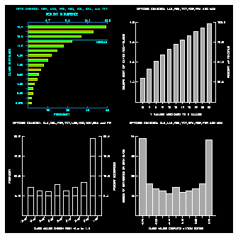
For comparisons or to save space, it is often advantageous to put more than one histogram on an output frame. To produce the following frame, HISTGR is called four times. On the first three calls, the frame is not advanced. After the fourth call, the frame is advanced.

Producing four histograms in one frame

Code segment 3 from thstgr.f

1       IFLAG = 0
2       NCLASS = 17
3       NPTS = 320
4       CALL HSTOPL('DEF=ON')
5       CALL HSTOPC('TIT=ON',
       + 'OPTS CHANGED: HOR, WIN, FRA, MED, COL, SPA, and TIT',9,3)
6       CALL HSTOPL('HOR=ON')
7       CALL HSTOPL('MED=ON')
8       ARR7(1) = 0.
9       ARR7(2) = .5
10      ARR7(3) = .5
11      ARR7(4) = 1.
12      CALL HSTOPR('WIN=ON',ARR7,4)
13      CALL HSTOPI('COL=ON',2,0,COLORS,8)
14      SPAC(1) = 3.0
15      SPAC(2) = 0.0
16      CALL HSTOPR('SPA=ON',SPAC,2)
17      CALL HSTOPL('FRA=OFF')
18      CALL HISTGR(DAT1, NDIM, NPTS, IFLAG, CLASS, NCLASS, WORK, NWRK)

Discussion

Lines 1 and 2 of code segment 3 from thstgr.f determine that the input dataset will be binned into 17 equal intervals.

Line 3 defines the size of the DAT1 array at 320 data values.

Line 4 resets all internal parameters to their default values.

Line 5 assigns a main title that relates which internal parameters are set for this histogram.

Line 6 requests that the histogram bars be drawn horizontally.

Line 7 requests a median line be drawn through the histogram.

Lines 8 through 12 set the location where this histogram will be drawn on a plotter frame that has a range of 0. to 1. in both dimensions. This particular call will place this histogram in the upper left quadrant.

Note: The process for putting multiple histograms on a page was to use the parameter WIN instead of using four calls to the SET routine of SPPS. This is because window and viewport scaling are done within the HISTGR routine, which would override any SET call put in the user code.

Line 13 sets colors for the graphics (not shown in the output here).

Lines 14 through 16 set the spacing between histogram bars.

Line 17 turns off the frame advance so that additional histograms can be drawn on the frame.

Line 18 generates the histogram shown in the upper left quadrant of the graphic.

Caveat: We regret the name choice of the parameter "WIN." In the terminology of GKS, this parameter should be called the viewport, not the window, since the viewport defines the plotting area on the output device.

Previous chapter                LLUs Home                    Next chapter